Category Archives: Student/Postdoc Blog

RRS Discovery – DY182: Icelandic basin and Irminger Sea

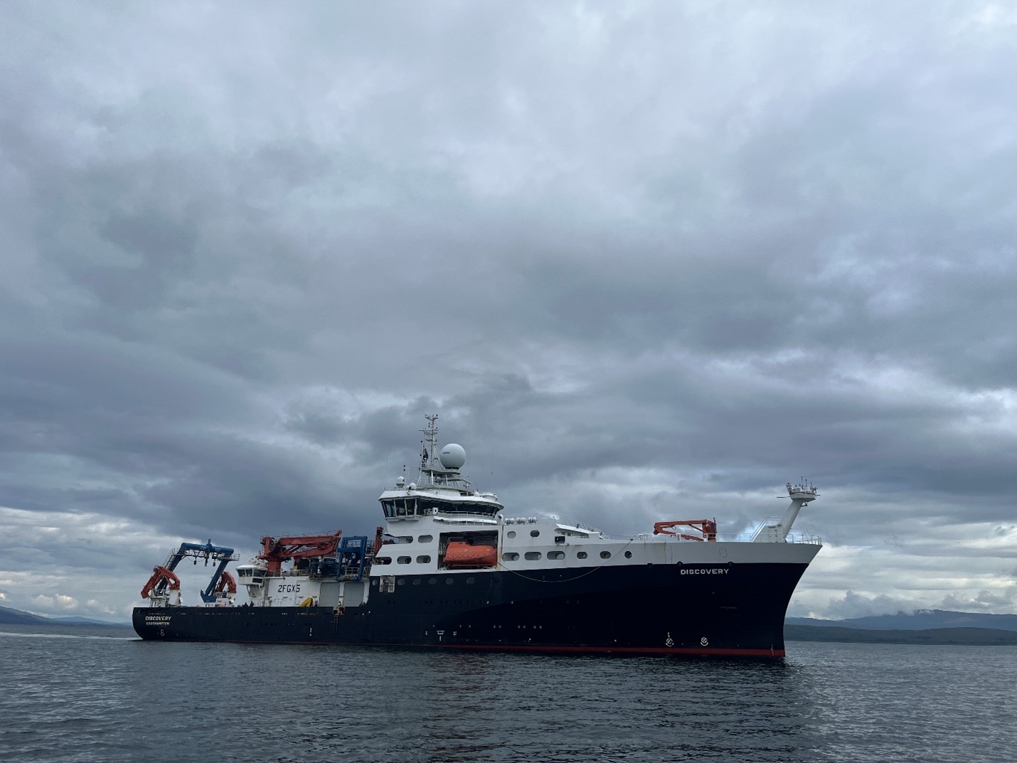
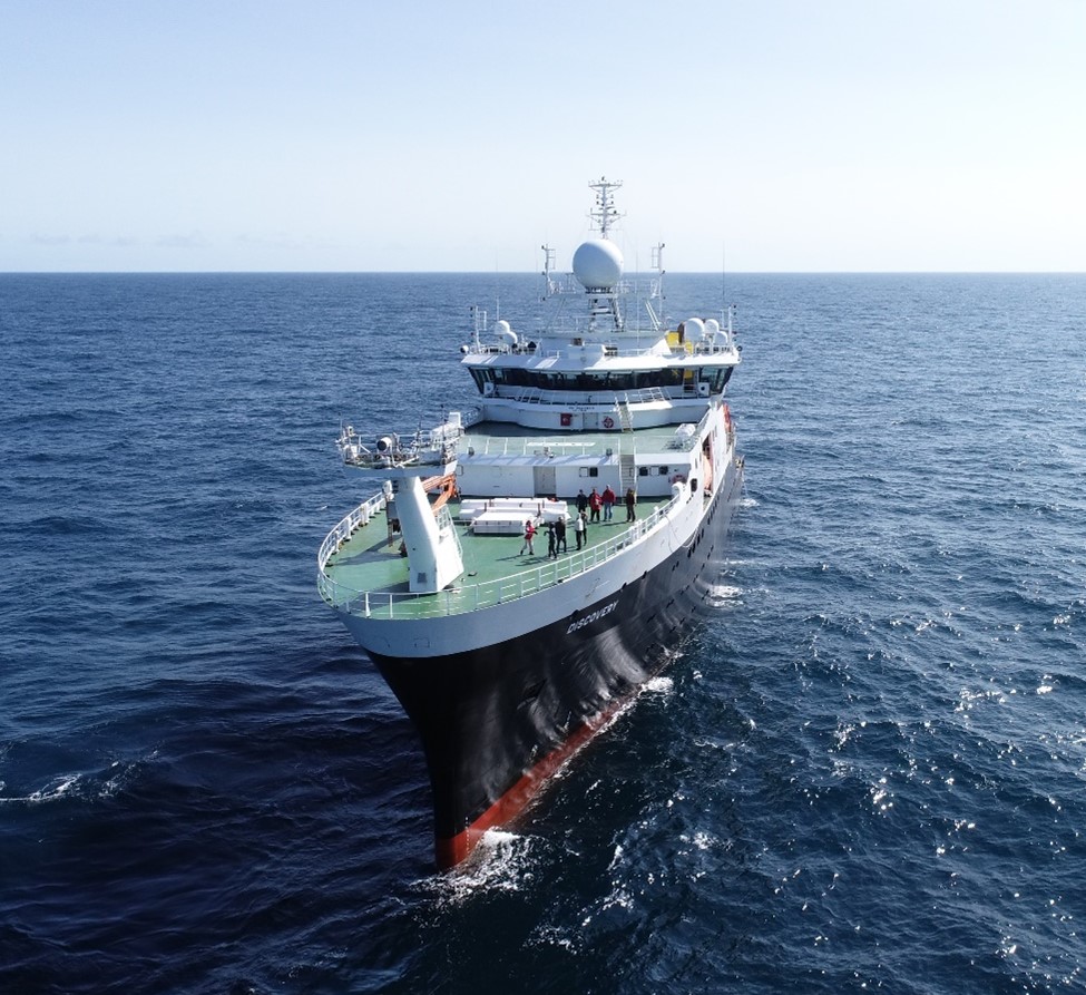
The RRS Discovery on a rare sunny day in the Irminger Sea, taken by the U. Miami drone.

Femke den Ouden – Student Utrecht University

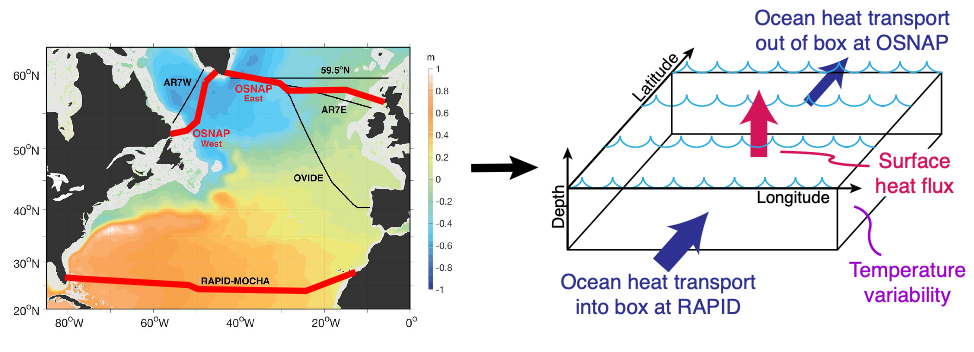
When I got an email from my Marine Sciences Master (Utrecht University) coordinator that you could sign up to join the DY182 cruise on the RRS Discovery, I didn’t hesitate. My main scientific interest is physical oceanography and the cryosphere and I just finished a course in which we elaborately discussed the AMOC and the OSNAP project. How amazing is it to actually experience a project and region like this, instead of only seeing it on a lecture screen?! When I heard that I would also be able to write my master thesis with NIOZ on the OSNAP data, I was even more excited to be able to experience the data collection hands on. I bought all the clothing needed for the expected cold and wind in the North Atlantic, did my safety training and medical exam and flew, together with my fellow students, to Reykjavik to start this adventure!
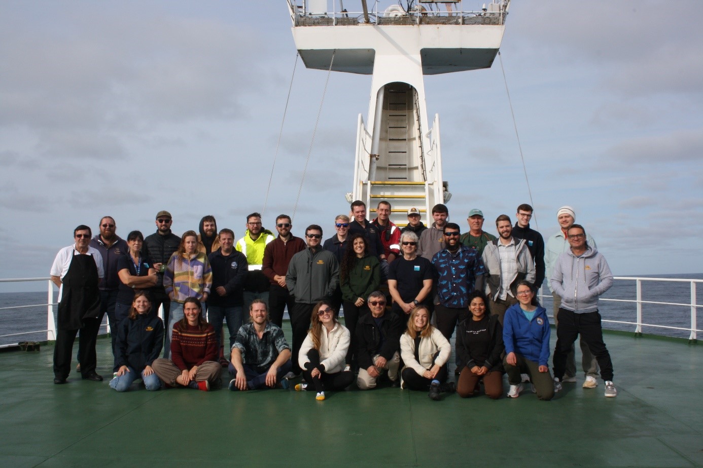
Group photo!

The DY182 cruise is shared between the University of Miami (moorings in the Icelandic basin, east of the Mid-Atlantic Ridge) and NIOZ (moorings in the Irminger sea, west of the Mid-Atlantic ridge). The University of Miami team is full of experienced seafarers: Tiago, chief scientist for the first time (lobbyist for a Brazilian barbeque on deck); Bill, the most experienced oceanographer and one of the founders of OSNAP (and the best cribbage teacher); and oceanographers and technicians Eduardo (who looks like a superhero in his safety harness), Cedric (likes to drink an IPA each night), Joe (No need for a spare anchor this time) and Houraa (showing exponential growth in her darts skills). From the Netherlands (NIOZ and Utrecht University) we came with a relatively inexperienced team. However, I feel like we bring a lot of enthusiasm and energy to the ship. Sasha, PhD student and the only one with real seagoing experience (can finally use his bike helmet); Emma, working on her virtual ship classroom (voluntarily wakes up at 4 in the morning); Claudia, having a do-over for the 2022 cruise (has a hate relationship with Microcats and a love relationship with Iceland); Laura, journalist of NRC writing an article on the AMOC (whose favourite moment of the day is sitting at the back deck with a book and cup of tea); Dave, NIOZ technician who impressed the whole ship with his efficient recoveries and deployments (can be found in the gym each day); and then lastly the students Aart (programming specialist and foosball star player) Ann (LOVES cleaning buoys with slimy marine life), Josefien (always does a happy dance when walking along the amazing food buffet), and me, Femke (the sports instructor of our team). And of course, the amazing technicians Ellis, Dean, Dave, John and Tom, and the rest of the crew!

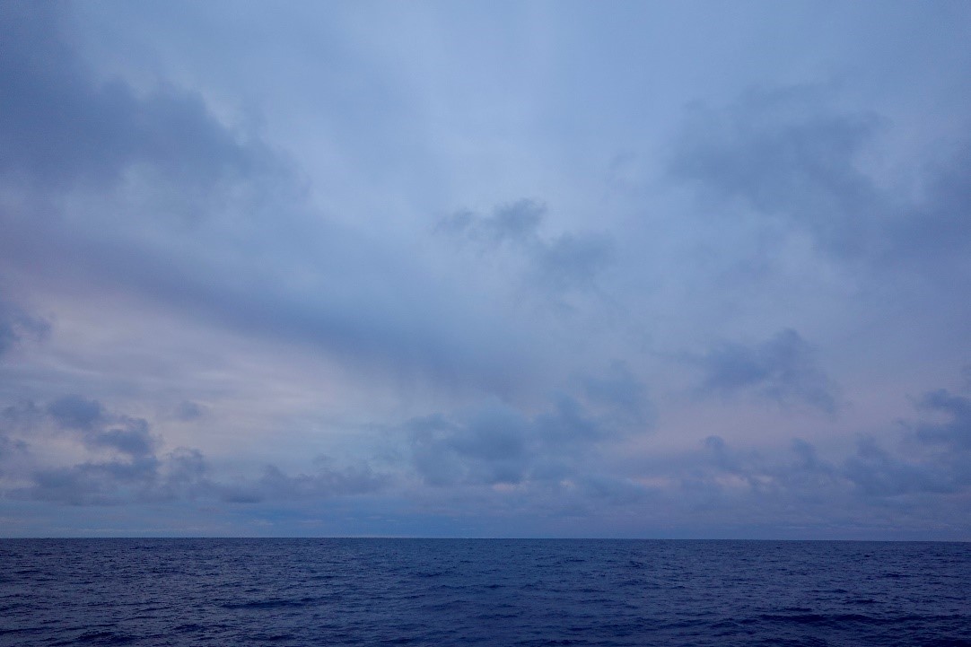
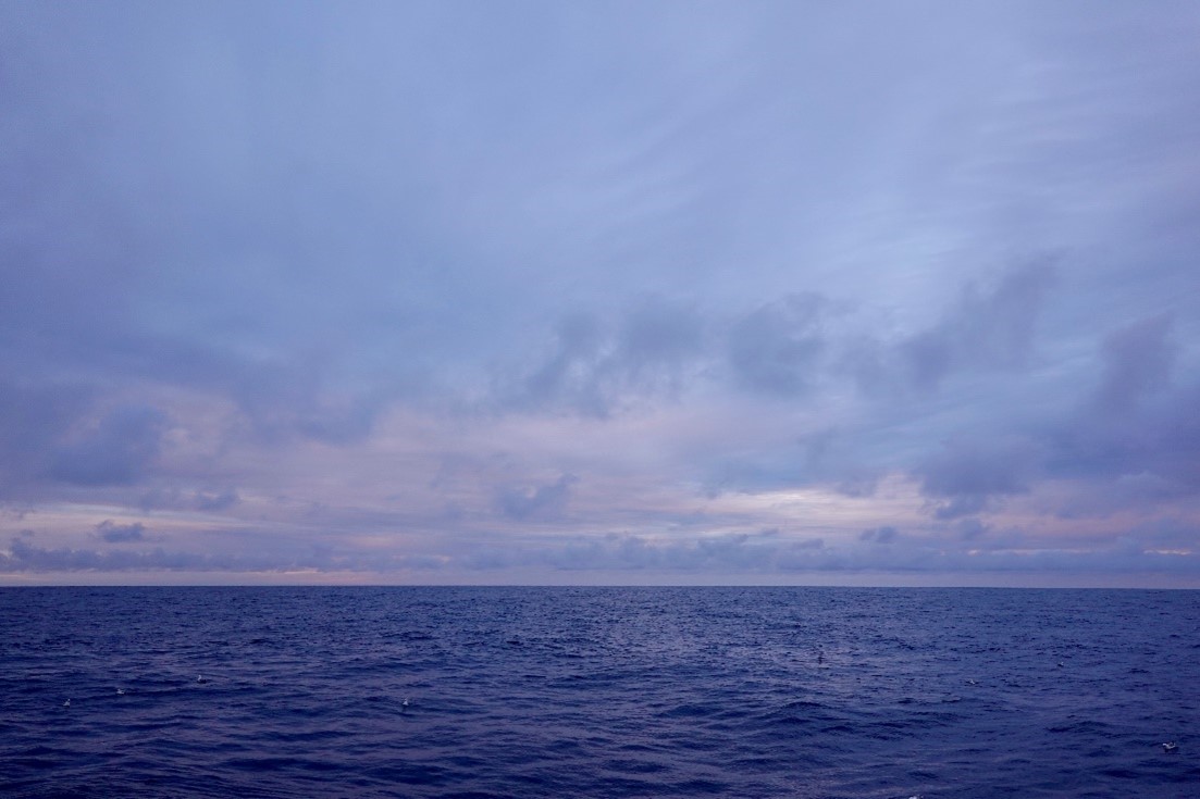
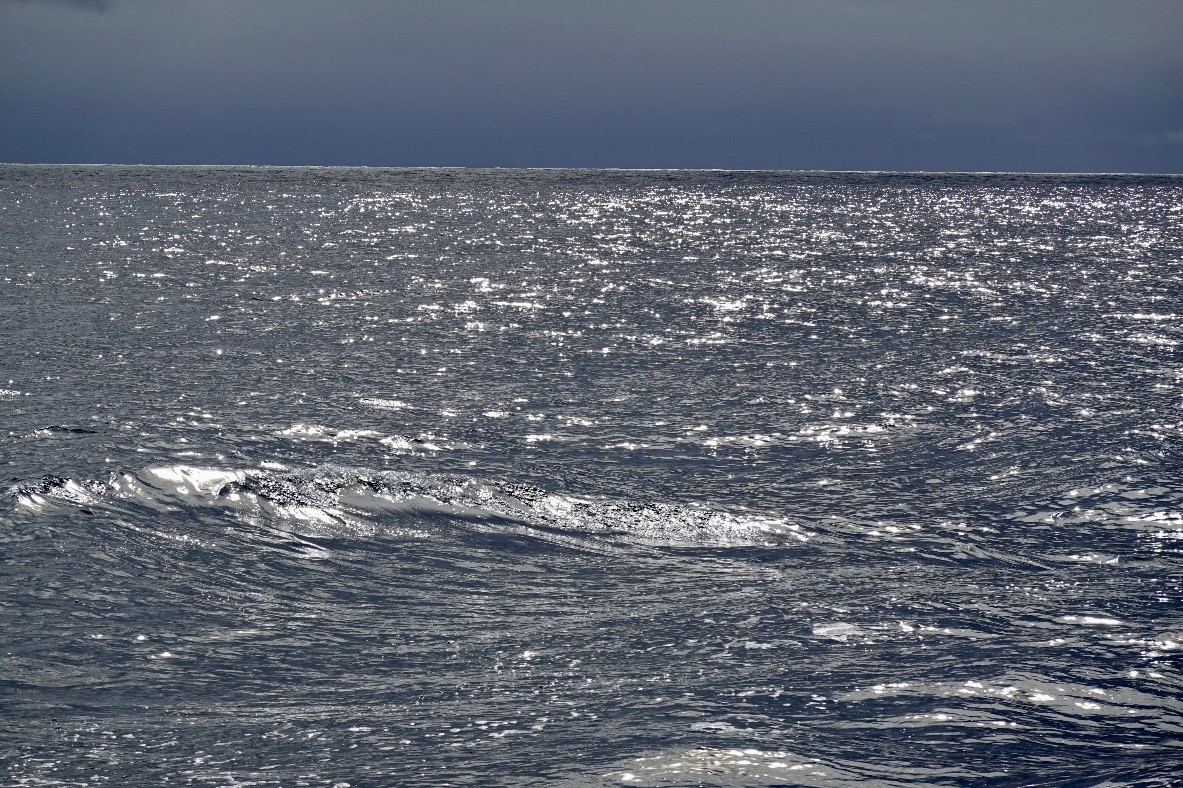
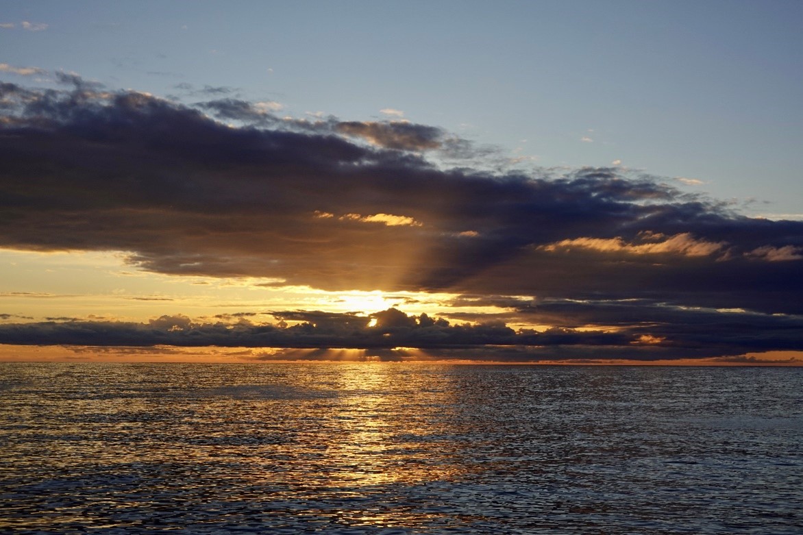
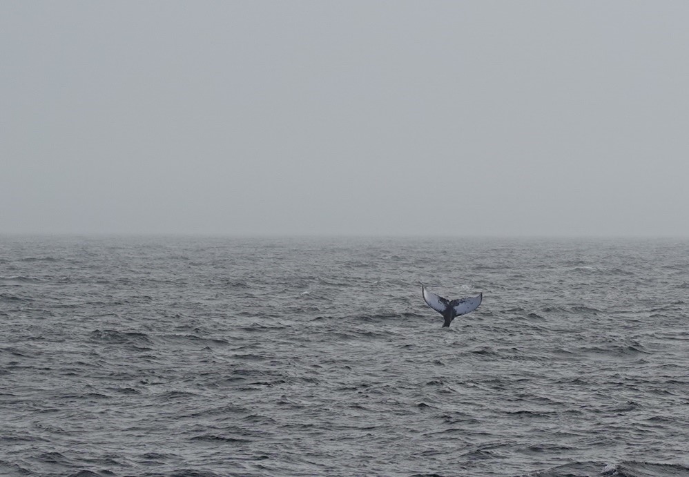
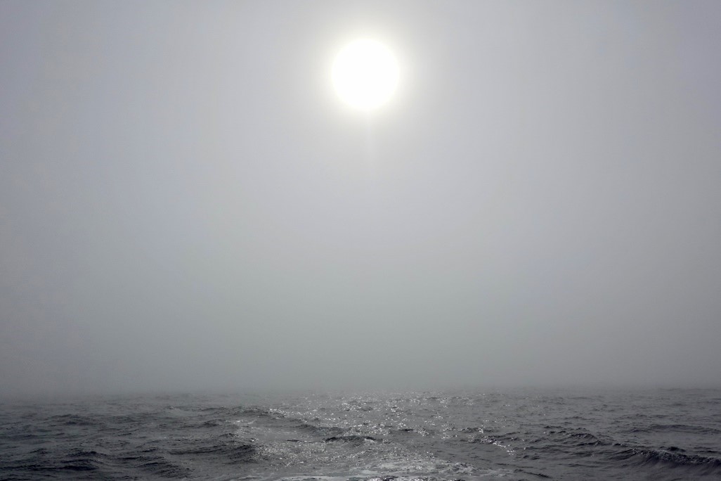
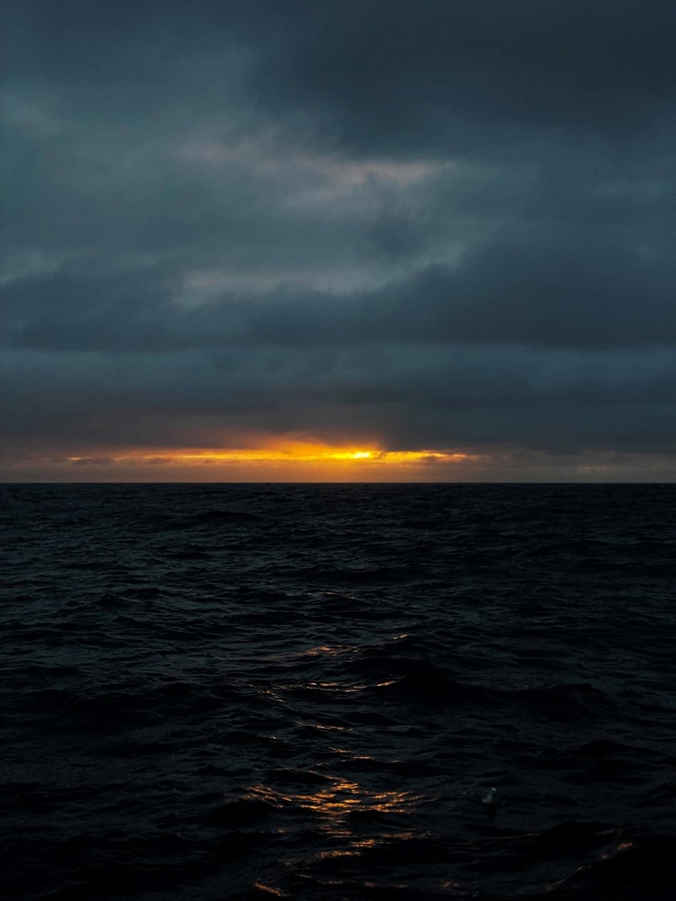
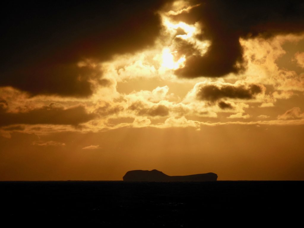
Besides the fact that the whales have been exceptionally absent this cruise, it has been amazing so far! We have had some very sunny days during which we could chill at the front or back deck, some great sunsets and sunrises, and not many fogs for which the Irminger sea is famous. I am very aware that I got very spoiled to have the Discovery as the ship for my first cruise. The ship is super stable so it took me only 2 days to grow my sea legs. Furthermore, we have the extreme luxury of CTD operators from the ship, which means that they do most of the CTD work. This gives us more time to learn about the moorings and their data. The food here is amazing, Peter, Neil, Tina and Tony make sure that all our hearts and stomachs desires are met. Luckily there is a relatively large sports gym, otherwise I would gain a kilo per week due to their amazing cooking and hospitality. The whole crew is amazing, they have made me feel welcome since day 1 and the Discovery has really started to feel like home in these past weeks.

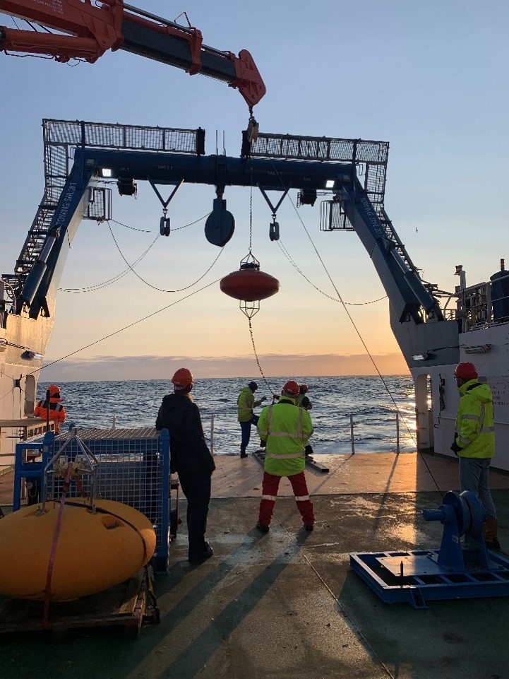
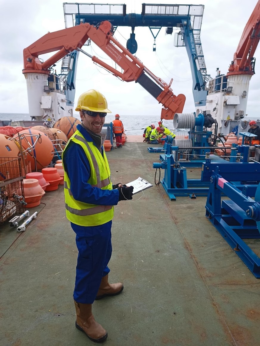
Early morning deployment of a NIOZ mooring.

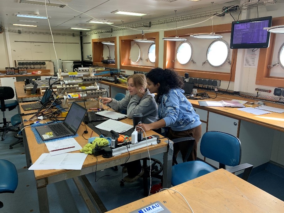
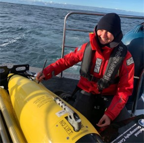
Femke and Ann programming and reading out instruments of the moorings.

Josefien’s typical day at the RRS Discovery

7:15 Waking up
My alarm goes off. The science cabins for the students are located on the Main Deck, which is on the same level as the sea, so I wake up with the sounds of waves splashing against my two small round windows.

7:30 Breakfast
The galley (the ship’s kitchen) is two floors up. Here, you find your typical English breakfast made by Peter and Neil. At 8:00 the first monitor check needs to be done, which only takes a couple minutes and needs to be done every two hours.

8:30 Science meeting
After breakfast we go one floor down to head towards the Main Lab. We meet up with the scientists, students, technicians and captain to discuss today’s research plan based on the weather forecast.

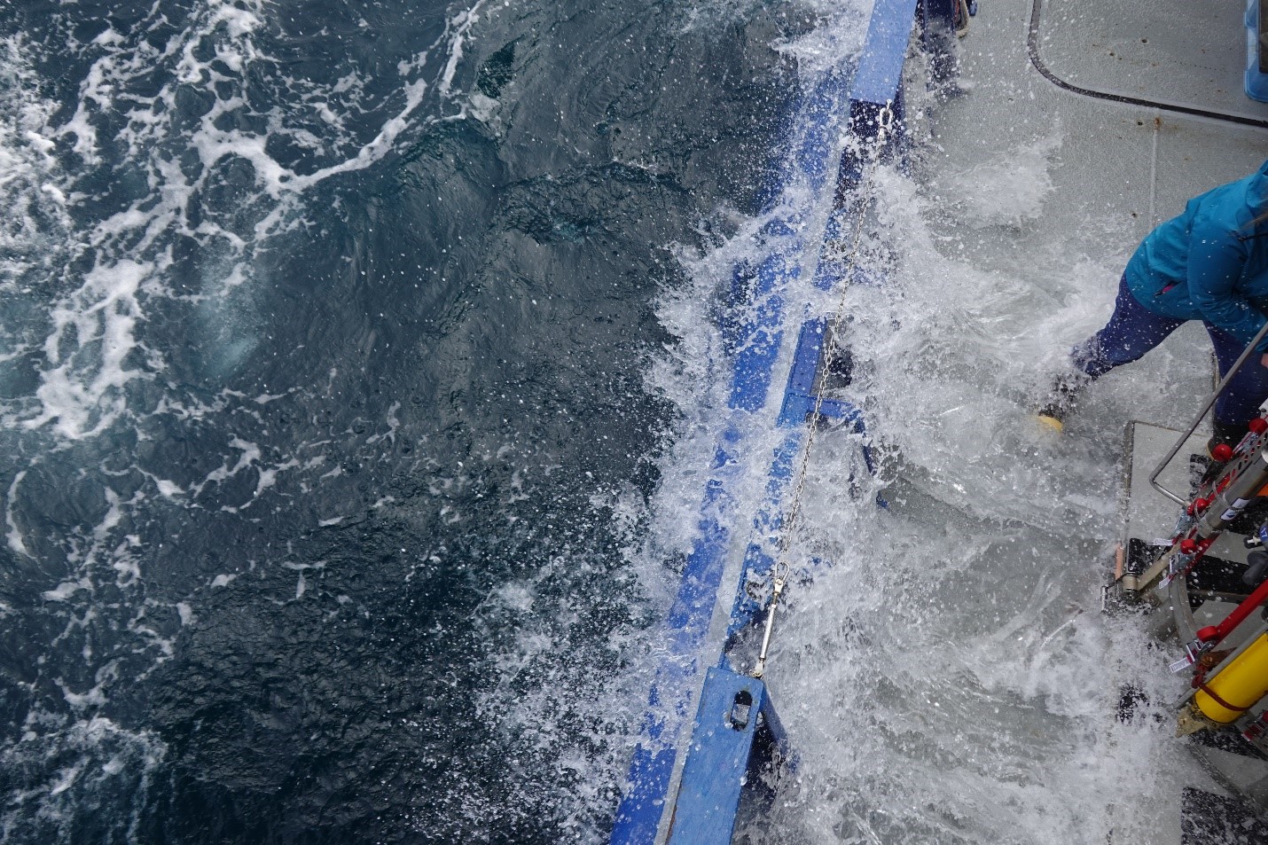
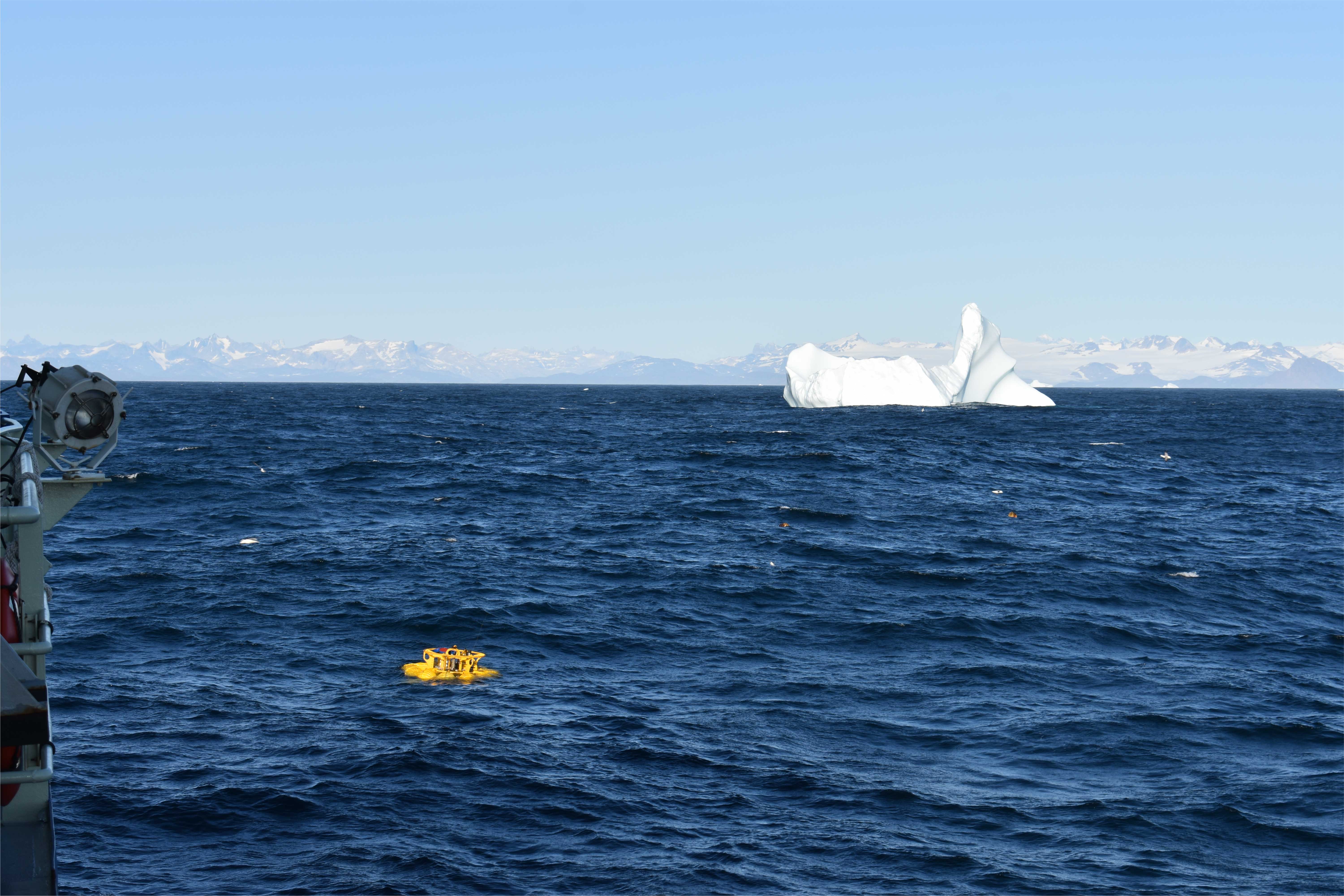
9:00 Mooring recovery
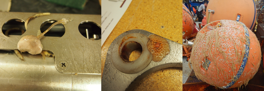
After spotting the big yellow buoys in the sea, the mooring is attached to the ship and cautiously lifted out of the water. Dave, our technician, carefully detaches each instrument; this takes a pretty long time since the mooring can be up to 2500 m. We help with cleaning the instruments (after two years in the ocean the devices are covered in algae and some slimy worms) and bring them inside to stop the logging and start reading out the data. In the rush of the mooring recovery, I forgot the monitor checks at 10:00, oops…

11:30 Lunch.
A nice and warm lunch is prepared for everybody. Way better than the slices of bread I would eat in the Netherlands! With so many options, your plate could look completely different from your neighbour’s.
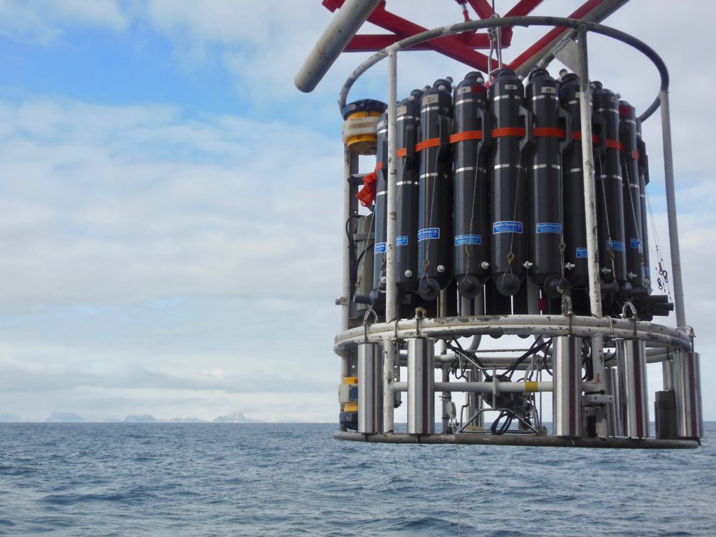
13:30 CTD
CTD time! The CTD Rosette collects water samples at different depths and measures the salinity, temperature and pressure on its way. We log the timing and coordinate position. Meanwhile, we begin programming the Microcats – devices that measure salinity, temperature, and conductivity – for a ‘Caldip.’ This calibration process compares the CTD measurements with those from the Microcats to determine their placement on the mooring line for deployment. Once the CTD is back on deck, we collect water samples and the technicians analyse them in the Salinity Lab.

15:30 Plankton
We deploy a plankton net to a depth of 50 meters. After the cruise, DNA analysis will be conducted on the collected plankton. To prevent contamination with human DNA, we handle the plankton net only with plastic gloves. In addition to lot of plankton, the catch also included fish larvae and miniature sea snails.

16:00 Sports
Together with Femke, Emma, Laura and technician Ellis, I am doing an intense workout in The Hold below the deck. Exercising is a lot harder on a moving ship, but way more fun!

17:30 Dinner and spare time
With the whole crew we have a nice dinner, especially the desserts are amazing. After dinner, we hang out in the bar, have a beer (max two per day is allowed), and play some games. Especially foosball and darts are popular. Unfortunately, Aart is on the winning hand with foosball… After watching an episode of Game of Thrones with some people, I go to my cabin to sleep.

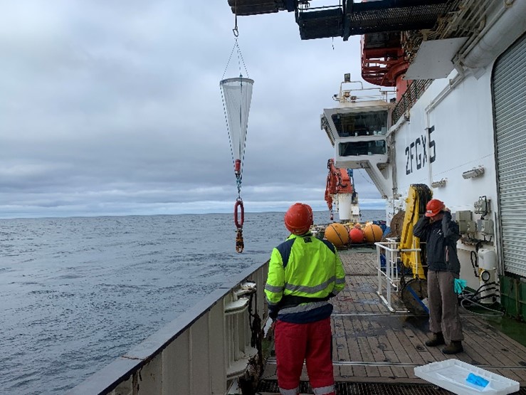
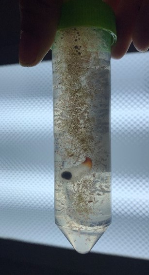
Daily plankton sampling.

Laura Bergshoef – Journalist NRC

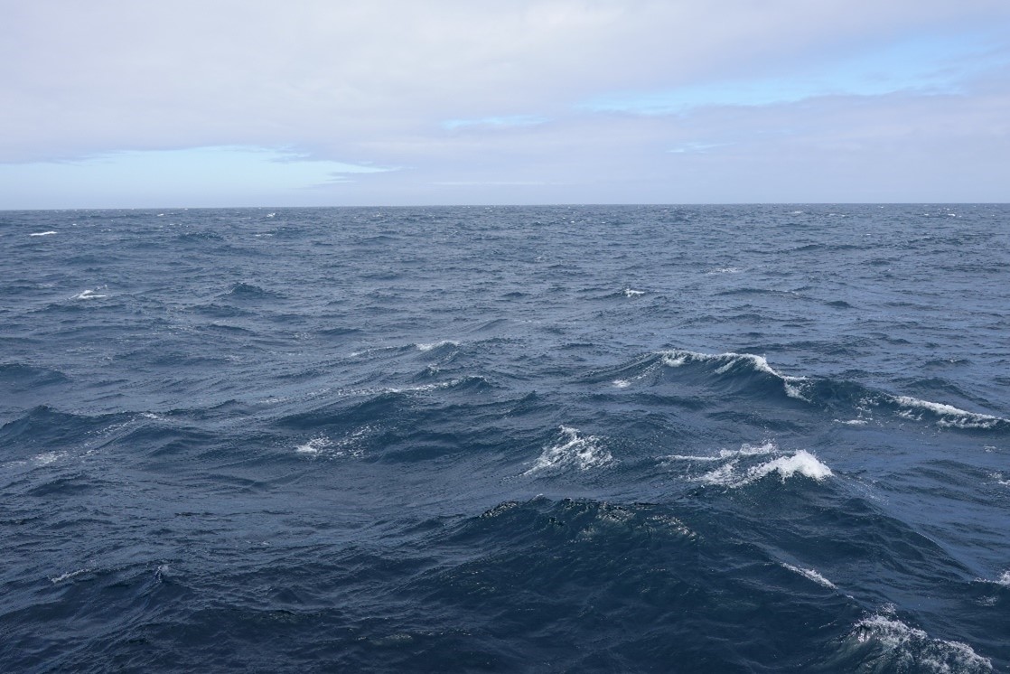
A day on the ship is never boring. Around us it might seem as an endless emptiness: just ocean, clouds and I only saw one other ship during the cruise. But inside the ship it’s never silent. Constantly you will hear ventilators, men with helmets talking though radio’s, rolling bottles and stories about pirates. I have been wandering around the ship a lot during day and night (and even saw the northern lights). Before coming on board I expected that life on sea will be lonely as we are so remotely. But the opposite is true. On the RRS Discovery – crossing the North Atlantic – we all eat, sport, watch Olympics, play games together as one big family on a Christmas holiday.

Surprisingly for me was that at night, the ship is controlled in complete darkness. Looking outside from the bridge, it felt like driving a car at night without any light. 

As a journalist I always try to get as close to my topic as possible. When Femke de Jong and I arranged a time and date for our newspaper interview and she joked that if I wanted to come as close to her work as possible I should join this cruise on the North Atlantic, I thought ‘why not’. As a climate scientist/oceanographer by training and author joining a cruise like this for a story is a dream come true. I think it’s one of the most special stories I will ever write.

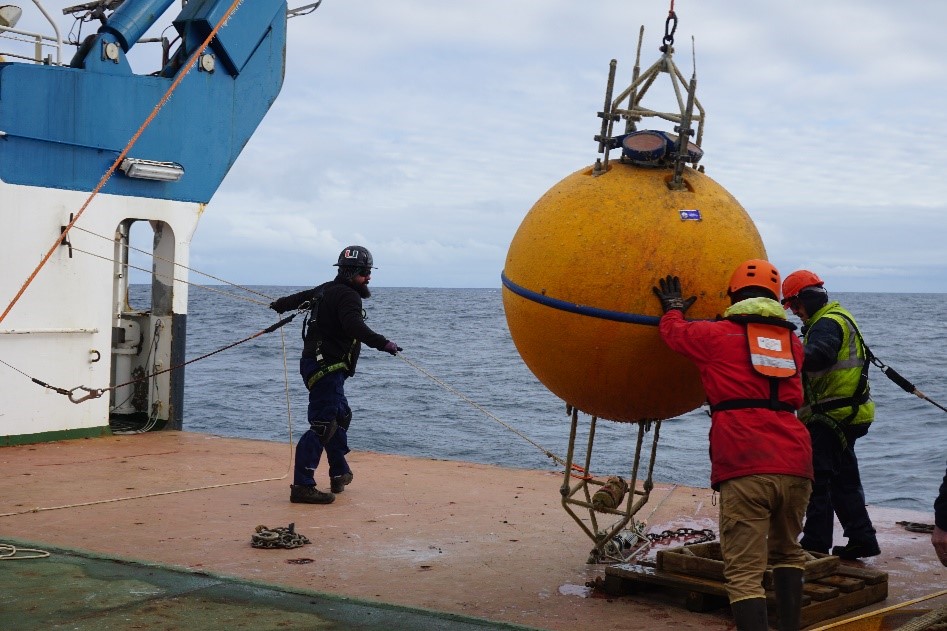
Recovery of the American moorings.

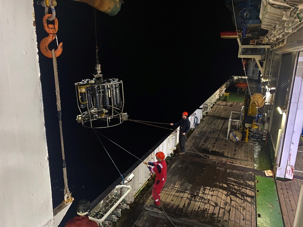
Nightly CTD stations


RRS Discovery – DY181, Aberdeen (UK) to Reykjavik (Iceland)

RRS Discovery before navigating the Sound of Mull, Westcoast Scottland.

The easternmost moorings of the OSNAP line are maintained by the UK project partners NOC (National Oceanography Center) and SAMS (Scottish Association for Marine Science) under the project AtlantiS. 2024 is a special anniversary year, as it will complete 10 years of OSNAP raw data. For me it is very special, as it is the first time I am leading a cruise. The UK cruise DY181 on RRS Discovery started in Aberdeen, UK on 3 July and we plan to arrive in Reykjavik, Iceland on the 28 July. As part of AtlantiS, we offered berths of opportunity on our OSNAP cruises to give early career scientists the chance to gather cruise experience or take part in the cruises with their own projects. In the following weeks, the successful candidates of the programme will introduce themselves here on the blog and share their cruise experience with you. For day-to-day updates we will post regularly under #DY181 on X. I hope you will enjoy the blog!

Kristin (SAMS, UK)


Me on deck monitoring the deployment of one of our moorings

Hello there, I’m Matt! I’m a physical oceanography research scientist from the National Oceanography Centre (NOC), Southampton. On board DY181, I am one of the physics watch leads. There are 3 physics watches, but what does this mean? We have 3 teams of physical oceanographers, meaning we can maintain operations 24 hours a day. I lead the 08:00 – 16:00 watch, but there is also a 16:00 – 00:00 followed by a 00:00 – 08:00.

What do we do? Every 4 hours, we do ‘the rounds’, which involves checking all the underway (permanently running) systems we use and make sure they are operating and logging correctly. At this time, we also take a surface seawater sample. We continually pump seawater into one of our labs and pass it through temperature and salinity sensors. Taking samples allows us to do checks to see if these sensors are operating correctly, within expected ranges.

The physics watch also oversee the deployment and recovery of our CTD rosette (conductivity-temperature-depth profiler). Our wonderful technicians who operate and maintain this piece of equipment trigger Niskin sampling bottles to close at depths that the chemistry and biology teams want to sample at. After the technicians hand over the data files from the CTD, the physics watch then process the data. While we do have some code that automates most of the process, we do have to manually tag any measurements that look like electrical noise.

We also help out the moorings team by assisting with logging instrument serial numbers that are used on the moorings. Or occasionally help with carrying or cleaning the instruments.

As you can see, life on board is very varied and there’s lots to keep us busy!

Dr Matt Clark


I am Anneke, a first-year PhD candidate at NOC Southampton. At NOC, I’m in the Marine Physics and Ocean Climate (MPOC) Department. In my research, I am using satellite altimetry in combination with in-situ measurements of temperature and salinity to obtain a basin-wide estimate of volume transport of the Atlantic Meridional Overturning Circulation (AMOC) and assess how that transport might change with latitude and how those changes might impact the regional climate.

On DY181, I am part of the Physics watch. My main tasks are taking salinity samples from the CTD-casts as well as the underway sampling system and doing some initial processing of the CTD data. Interestingly (Or lazily😉), we don’t analyse the salinity samples ourselves. This is almost exclusively done by the technicians on-board. Maybe because the salinometer can be a little temperamental…

I am also the designated Marine Mammal Observer (MMO). MMOs make sure that the acoustic systems we carry on board to measure depth and plot bathymetric profiles (single-mean and multi-beam echosounders) don’t pose a risk to marine mammals, specifically the organs that allow them to do echolocation. Usually, this is not a problem as we operate the echosounders on a continuous basis so there is no sudden exposure to sound for any mammals in the vicinity. During certain science operations, however, the acoustic signals from the echosounders can interfere. This is the case during the release of moorings when recovering, or when determining the position of a mooring after deployment (ranging and trilateration), for example. In those cases, the echosounders have to be switched off and my job is to make sure they are not switched off for too long, to avoid this sudden exposure to sound of any mammals when we switch them back on again. If they were switched off for longer than 10 minutes, I’d have to keep a mammal watch on the bridge to check for presence of any mammals in the vicinity and only if there was none could we gradually switch on the acoustic systems again. Really all I do is start and stop 9-minute alarms and log the times that we switch the echosounders on and off, but everyone involved in ranging and trilateration of moorings is aware of these limitations anyway, so it is a pretty straight-forward process (hopefully I’m not jinxing it, as we still have a few moorings to recover and deploy at the time of me writing this :o). Because I am the MMO, I have been assigned to the daytime watch (just in case I did have to do a mammal watch), which comes with some perks😊 First of all, I don’t have to adjust to a nocturnal rhythm, which can be difficult (if not utterly horrifying the moment you realise you may miss out on Full English breakfast or Sunday roast :o); but it also means I can learn lots and get involved with the other science operations on-board that are usually only carried out during daylight, such as the recovery and deployment of moorings and Argo floats, which is exciting! I think this diversity might be the best part for me on this research cruise!

Anneke Sperling

OSNAP (Ocean Sentiments, or Newly Arisen Ponderings)

By Ayden Schirmacher, Boston University student

As someone who grew up on the west coast of the United States, the ocean has always been a part of me. I think it was something I took for granted, that it was always going to be there, and maybe I didn’t visit as much as I should have. But as with many young people, there are often any number of other things more pressing than staring into a watery horizon. As I have gotten older though, I find myself understanding more and more why everyone from poets to real estate moguls to scientists have been captivated by the ocean, recognizing its value and potential.

I’ve had time in excess during this cruise, given that our transit was a substantial eight days from Woods Hole to the Irminger Sea, and most of my work on the ship had to do with CTD casts. Yet for this whole time, there have been very few moments of silence, maybe three colorful sunsets, and only a few days of smooth waters. The sun has been coming out more recently – my new favorite color is just “ocean” – but for the most part we have been in a dense fog on choppy seas. The result is a veritable cocoon of water, both underneath and around us, narrowing the possibility of sight to what is right in front of you. Still it is amazing what you can see in that tiny bubble – fin whales approaching from the starboard side! Fulmars flying behind! The buoy is bobbing away into the fog, can you see it go? I love it.

As a first-time sea-goer and student, I have learned so much and had my eyes opened to some pretty amazing work. It has made me think a lot about the reciprocal relationship of humanity to the seas, a relationship which still contributes to the sustainability of the global population today through providing opportunities for livelihoods and resources. However, as we already know, it has been impacted by climate change. There are rising sea levels already posing a real danger to millions of people, on top of the decimation of marine ecosystems and biodiversity.

There is an idea that I love, that climate change impacts life on the planet, but not the existence of said planet. It is a horrific tragedy, the destruction our species is wreaking, but I find there is something comforting about the knowledge that the planet, and its oceans, will be around a lot longer than we can comprehend. The permanence of it all is awe-inspiring. It’s an idea that has big implications and is a little hard to wrap one’s head around sometimes. But it becomes a lot easier to get the point when on a not-insignificantly sized vessel, getting rocked around by 3-meter waves, which in the grand scheme of things isn’t even that bad.

That being said, it’s obvious that the destruction of life on this planet is awful. So it gives me hope that people are actively working to study and preserve the ocean and its systems. The operations carried out by the teams aboard the Armstrong are complex and difficult, but so far have been

conducted with a capability and efficiency that are most admirable. From the deck crew to the Chief Scientist, the impression is of a well-oiled machine actively working to ensure the scientific community and the public have access to the best data possible. Oceanography is a very special facet of that human-sea relationship: a way of understanding, but the ocean fights you while doing it. You have to earn the knowledge, which I think is quite beautiful.

I like knowing that while we may be floating in our little fog bubble in the Irminger Sea, the implications and impacts of the work being done here are far-reaching and important. Thus far, I have had one of the best months of my life. The ocean is certainly inspiring, both of fascination and a healthy dose of fear, and I am glad to be a part of at least a small part of the work being done to understand it better.

June 13, 2024 – The first rough seas of the trip. Image taken from the starboard side of the ship, facing the bow. Seas this day were an average of 2.5m.

June 13, 2024 – Waves crashing over the side of the ship as work is being done on the CTD/Niskin rosette. Sampling in these conditions is not for the faint of heart!

June 13, 2024 – Panoramic view of the waves during the middle of the day. Fast winds make for the whitecaps on the waves.

June 16, 2024 – Even though they don’t like to land on the ship, the sea birds frequent the skies and seas around us. Sometimes they get close enough to see every feather!

June 20, 2024 – Occasionally the sun will be out during the day, but tends to go away in the afternoon behind fog. On this day, the clouds were broken enough to see some light, and the clouds ended up looking like an abstract version of the Northern Lights.

June 20, 2024 – This far north, the skies may not have the traditional orange sunsets, but the purples are just as beautiful. The rarity of having a colorful sunset just makes you appreciate it even more!

June 21, 2024 – My new favorite color is “ocean”. On this day, the sun came out in slivers, but lit up the sea so that it became a beautiful blue/purple/silver color.

June 03, 2024 – the last “real” sunset of the trip, on our second day at sea. Ever since then, we have been too far north to really see the sun go down at a reasonable hour.

June 04, 2024 – A humpback whale flips its tail up at us as we sail past. 

June 06, 2024 – The dense fog creating a grey wall. But it’s beautiful in its own way.

June 22, 2024 – Sometimes the sun peeks through if you can catch it at the right time.

Neil Armstrong – Woods Hole

By Emma Brown, Boston College student

We arrived in Woods Hole! We immediately began lashing down anything that exciting seas might send sliding. This included various boxes of scientific materials, including our toolbox, with bungee cords and ratchet straps. Our filtration system was placed on a sticky mat and bungee corded in both directions. Other boxes, some meant to hold future samples, were lashed in place in the cooler atop metal racks.

This morning, all hands were on deck to help board stores! A large crane lowered cloth nets bulging with boxes of goods into the ship, directed by crew members in hardhats. Once the goods had reached the floor, these crew members freed the net from the holding hooks and cut the boxes loose from their plastic packaging. Then, almost all crew members and scientific personnel formed a passing chain to help load frozen, refrigerated, and fresh stores onto the Neil Armstrong. The process was amazing! Everyone worked as an oiled machine as the galley quickly filled with boxes upon boxes of assorted goods. Our second mate, Chrissy, worked as fast as she could to fit these boxes jenga-style into a food elevator to put them into the ship’s massive freezer/refrigerator.

We began our journey across the Atlantic! We were on the boat by 9 am and met for a team meeting and safety training at 10 in the main lab. The 1st mate, Chris, explained the protocols for fire and abandoned ship. Ayden demonstrated how to don a life-saving wetsuit. It’s not very complicated after you’ve been shown how to do it (I also had to try mine). I was just a half inch too tall for a small- apparently, they’re made for people exactly 5’4 and under. The next size up must be made for people about eight feet tall because I was practically swimming in it. One must lay this suit on the floor to climb into it, one limb at a time. Chrissy, the third mate, helped me get my arms and legs inside. The suit may be zipped up past one’s chin and a strap is placed over the lower part of one’s face. The final step is to squeeze all the air out by crouching and hugging one’s knees. The suits are enormous and clunky beyond imagination, but life-saving in an emergency.

At noon precisely, the boat was pushed away from the dock and we all waved goodbye to those we were leaving behind on land. Following departure, we did drills for emergencies. For a fire, everyone met in the main lab. For abandoned ships, top bunk people rendezvoused at the port side of our vessel and bottom bunk people convened at the starboard side. Later in the evening, the boat stopped for our first CTD cast! In hard hats, steel-toe boots, and bibs (foul weather gear, lacking the jacket), we undid the ratchet straps anchoring the CTD in place on the deck. A well-oiled crane picked the CTD up on a thick cable. The tension in the cable was visible via a screen well over our heads. The tension rapidly increased as the CTD was lowered over the water. We popped all of the Niskin bottles open on top and bottom. These “fired”- aka, closed- once the CTD reached the desired depth at 165 meters down.

The machine was then slowly pulled back to the surface on its cable and gently lowered onto the boat, dripping seawater. We quickly strapped it back to the deck. Then, we tested each bottle to be “leakers,” meaning it’s a Niskin that did close properly on the way up therefore, it’s bad water and can’t be used for science. We took samples for DOC (dissolved organic carbon) and POC (particulate organic carbon). Both involve rinsing the sampling bottle and cap out 3x, then filling to the top with seawater from the desired Niskin. Immediately after, in the lab, we practiced filtering both types of samples.

Photo: The author spends free time on the transit painting and drawing each day.

A closed heat budget for the mid-latitude North Atlantic?!

by Nick Foukal

Now that the OSNAP and RAPID arrays are running concurrently, an obvious question arises: can we close a heat budget for the mid-latitude North Atlantic? A heat budget is a very simple concept – let us pretend that the ocean between RAPID and OSNAP is a box with an ocean flux coming into the southern boundary (at RAPID), another going out of the northern boundary (at OSNAP), and surface fluxes exiting through the top (Fig. 1). The sum of the oceanic fluxes and surface fluxes should equal the change in the temperature of the box, meaning the heat budget is “closed” (see equation below). This is a useful exercise because determining whether the ocean temperature variability is caused by ocean dynamics or surface fluxes gives us a better idea of how the system will evolve in the future. Though this task of closing heat budgets may seem incredibly simple to the lay audience, it has never been done before for a region as large and important as the mid-latitude North Atlantic.

Ocean temperature variability = surface heat flux + ocean heat transport divergence

Figure 1 – (left) RAPID and OSNAP lines in the North Atlantic (red lines) and time-mean sea-surface height (colors). Figure adapted from Lozier et al. (2019). (right) Simplified box representation of the mid-latitude North Atlantic heat budget with ocean heat fluxes into the box at RAPID, out of the box at OSNAP, and a net surface heat flux out of the ocean.

To close the heat budget with observations, we need reliable measurements of all three terms. There are very reliable reconstructions of ocean temperature variability (from satellites and Argo floats), decent guesses of the surface fluxes (primarily derived from satellites on these scales), but very poor estimates of the ocean heat transports. The processes that govern ocean heat transport operate on such small scales that they are difficult to measure in the absence of dedicated in situ arrays. Consequently, what is often done in the literature is the ocean heat transport term is inferred from the difference between the other two terms, and the heat budget is assumed to close. But this is not completely satisfactory because the surface heat fluxes typically have significant uncertainties (more on that later), so relying on them as the “known” component in a heat budget doesn’t inspire confidence in the result.

This is where the OSNAP and RAPID lines come in – they offer an unprecedented opportunity to bound the ocean heat transports over a large region. Never before has a region of this size been this densely sampled. This means that we no longer have to rely on the surface fluxes and conservation laws to close the budget. By knowing all three terms of the heat budget, we can assess how closely we can close the budget… essentially how well do our measurements from independent platforms agree with one another?

There is still one hurdle to overcome in this problem, and that is the uncertainty in surface heat fluxes. This is not a new problem to the field, it has plagued both oceanographic and atmospheric studies for decades. There are two well-known unknowns in surface heat fluxes: (1) the time variability between different surface fluxes data sets do not agree with one another and (2) the global surface fluxes averaged over time do not integrate to what we would expect from observed ocean warming rates. I recently ran into the former concern in a recent paper (Foukal and Lozier, 2018) where we looked at the heat budget for the eastern North Atlantic subpolar gyre in two models, and the end result of our study depended on which surface flux data set we used. With respect to the latter concern, we know that from rates of global ocean warming, the global net surface heat flux must be around 0.5-1 W/m2, yet some surface heat flux products sum to almost 25 W/m2globally (Yu, 2019, Cronin et al., 2019). So there is good reason to doubt both the mean and the variability in surface fluxes, which is not encouraging.

As a taste of this uncertainty, I compiled time series of the surface fluxes over the region bounded by RAPID and OSNAP for three different surface flux products (Fig. 2). To give a rough idea of what we should expect from the surface fluxes, the oceanic heat flux into the box through RAPID from 2004-2007 was 1.33 +/- 0.40 PW (Johns et al., 2011), and the oceanic heat flux out of the box through OSNAP from 2014-2016 was 0.45 +/- 0.02 PW (Lozier et al., 2019). If we assume that these two time periods are representative of the long-term mean, and that the ocean is in steady-state (i.e. the temperature variability is zero when time-averaged), then we should expect the surface heat fluxes to equal the difference between the two oceanic heat fluxes, or 0.88 PW out of the box. Instead, the mean surface heat fluxes are 0.43 PW (ERA5), 0.11 PW (OAFlux), and 0.11 PW (NOCS), all directed out of the box. While it is encouraging that the sign of the fluxes is correct in all three products and that two of the products agree with one another, it also means that somewhere between 0.45-0.77 PW is missing in our heat budget. To put this another way, at least an entire OSNAP of heat transport is missing from this budget, and maybe more. Furthermore, the only statistically-significant correlation between the time series is a relatively weak (r=0.56) connection between the annually-averaged ERA5 and OAFlux. NOCS had no significant correlations to either of the other two. So overall, the spread between the three data products, their lack of coherent variability, and their disagreement in the mean with the net ocean heat divergence does not inspire confidence that we can close a heat budget for the mid-latitude North Atlantic.

Figure 2. Surface heat flux variability integrated over the region between the RAPID and OSNAP arrays in three surface flux products (positive downward; units are petawatts = 1015 W). The thin lines are at monthly resolution, and the thick lines are annually-averaged. The seasonal cycles are removed from the monthly data to consider the non-seasonal variability. The ERA5 (Copernicus Climate Change Service) reanalysis is a ¼° product covering 1979-2018. The OAFlux (Yu et al., 2008) data set covers 1984-2009 at 1° resolution. The NOCS (Berry and Kent, 2011) surface heat fluxes are produced at 1° resolution for the period 1973-2014. The RAPID and OSNAP time periods are shown in the bottom right.

Before we lose hope, it is worth revisiting some of our methods and assumptions: (1) can we really compare the RAPID meridional heat transport from 2004 to 2007 to the more recent RAPID data from 2014 to 2016? Are the heat transports at RAPID from 2014 to 2016 perhaps lower than 1.33 PW? Lozier et al. (2019) report a net heat transport divergence of 0.80 PW between RAPID and OSNAP for the 2014 to 2016 period, which accounts for 0.08 PW of the missing heat fluxes. (2) Can we prioritize the ERA5 time series because it is the highest resolution and the most recently-released of the three products? During the 21 months of published OSNAP data, the mean ERA5 heat flux was 0.57 PW, or 33% larger than the 1979-2018 mean. So if we believe ERA5 over OAFlux and NOCS, then we are only missing 0.23 PW (0.80 PW – 0.57 PW), or only half of an OSNAP! (3) Maybe the ocean was not in steady-state for the OSNAP period (2014-2016), and instead of zero temperature change, the ocean actually warmed considerably? This is a bit of a stretch, as 0.23 PW would be a lot of warming. But it would be worth considering how much the region did warm over this time period to see how it affects the heat budget. After all, each of these heat transports has associated error bars, so maybe we can get close enough so that the error bars explain the residual? I will leave this analysis to further work, as this blog post is getting closer and closer to possible publication material…

So where does this exercise leave us? Surface heat fluxes are certainly a wild-card, but recent improvements (ERA5) seem to be trending in the right direction. In the next few years, OAFlux will be updated with higher resolution, so it would be worth checking if that time series validates the higher surface flux values of ERA5. Finally, I am contractually obligated to mention that continuation of the OSNAP line in the coming years is absolutely critical to closing the heat budget for the mid-latitude North Atlantic. A longer time series would improve our assumption of steady-state in the temperature variability and provide a better understanding of the inherent time scales of the overturning in the subpolar North Atlantic.


References:

Berry, D. I. and E. C. Kent (2011). Air-sea fluxes from ICOADS: the construction of a new gridded dataset with uncertainty estimates. International Journal of Climatology, 31, 987-1001.

Cronin, M. F. and 26 co-authors (2019). Air-Sea Fluxes With a Focus on Heat and Momentum, Frontiers in Marine Science, 6, 430, doi:10.3389/fmars.2019.00430.

Foukal, N. P. and M. S. Lozier (2018). Examining the origins of ocean heat content variability in the eastern North Atlantic subpolar gyre, Geophysical Research Letters, 45, 40, 11275-11283.

Johns, W. E., M. O. Baringer, L. M. Beal, S. A. Cunningham, T. Kanzow, H. L. Bryden, J. J. M. Hirschi, J. Martotzke, C. S. Meinen, B. Shaw, and R. Curry (2011). Continuous, Array-based estimates of Atlantic ocean heat transport at 26.5°N, Journal of Climate, 24, 2429-2449.

Lozier, M. S. and 37 co-authors (2019). A sea change in our view of overturning in the subpolar North Atlantic, Science, 363, 516-521.

Yu, L., X. Jin, and R. A. Weller (2008). Multidecade Global Flux Datasets from the Objectively Analyzed Air-se Fluxes (OAFlux) Project: Latent and sensible heat fluxes, ocean evaporation, and related surface meteorological variables. Woods Hole Oceanographic Institution, OAFlux Project Technical Report. OA-2008-01, 64pp. Woods Hole, Massachusetts.

Yu, L. (2019). Global Air-Sea Fluxes of Heat, Fresh water, and Momentum: Energy Budget Closure and Unanswered Questions, Annual Review of Marine Science, 11, 227-248.


Recently graduated: end of an amazing adventure and beginning of another

by Tillys Petit

My last contribution on this blog reminded the importance of in-situ data measurements on the evaluation of numerical modeling used to predict climate. As part of my PhD thesis, I had the chance to record, process and analyze observations across and along the Reykjanes Ridge within the framework of the RREX project. It included an experience at sea during the RREX cruise in 2017, which was an amazing human and scientific experience. Now that my PhD ended, I would like to tell you about the scientific results that were obtained. 

During my PhD, I studied the connection between the Iceland Basin and the Irminger Sea through the Reykjanes Ridge. A main result was to describe and quantify the top-to-bottom transport of the subpolar gyre that crossed the Reykjanes Ridge during the summer 2015. These results highlighted interconnection between the two main along-ridge currents: the southwestward East Reykjanes Ridge Current (ERRC) in the Iceland Basin and the northeastward Irminger Current (IC) in the Irminger Sea. From about 56 to 63°N, the hydrological properties, structures and transports of the ERRC and IC consistently evolved as they flowed along the Reykjanes Ridge. During my PhD, I showed that these latitudinal evolutions were due to flows connecting the ERRC and IC at specific locations through the complex bathymetry of the ridge, but also to significant connections between these currents and the interiors of the basins. These results highlighted a more complex circulation in the vicinity of the Reykjanes Ridge than it was assumed.

From three different cruises and Argo floats, I also investigated the deep circulation and properties of overflow water through the deepest sills of the Bight Fracture Zone. At the end of my PhD, I showed the strong variability of its transport and property over time by comparing three successive years. Now, I think that it could be interesting to continue this study and to better understand the variability of overflow water at higher frequency. As a continuity of my PhD, I am thus exciting to investigate the variability and linkage between the overflow water transports and properties across the Iceland-Scotland Ridge and the Denmark Strait as part of my postdoctoral position. These inflows from the Nordic Seas feed the lower limb of the Meridional Overturning Circulation and are crucial to characterize the variability of the North-Atlantic subpolar gyre. I am excited to fulfil this study by using the OSNAP array that provides new and key measurements of the AMOC, and also to move in USA for a new beautiful and rewarding postdoctoral experience.

My career path in physical oceanography and climate science

by Yavor Kostov

The end of the year is a time to reflect on the past and make long-term plans for our future. Some readers of this blog, especially our young audience, may be considering a career in oceanography or climate science. I will tell you my story: what motivated me to join this field and the factors that shaped my career path.

My first encounter with physical oceanography was 14 years ago, at an international summer school where I learned basic gravity wave dynamics. Fluid motion fascinated me and sparked a lasting interest in the field. The following year I was on my high school team for the International Young Physicists’ Tournament (IYPT). Within our team, I was responsible for problems related to fluid dynamics.

By the time I began my undergrad studies, I was already very interested in modeling the environment. I also realized that to do well in the natural sciences, I should expand my background in math. So I majored in Applied Mathematics, but I also took physics courses. As an undergrad, I did different research projects applying mathematical methods to study the environment. For example, my senior thesis was on modeling the El Niño / La Niña phenomenon.

Nine years ago, I decided to do a Ph.D. in climatology and oceanography. I became interested in the field because I wanted to do research in an area of science that is socially significant. Nature has direct impact on humankind.  At the same time, climate science and oceanography attracted me because many fundamental questions in our field remain unresolved.

My Ph.D. and postdoc research has explored the large-scale ocean circulation and its impact on global and regional climate. I have studied various parts of the World Ocean: the North Atlantic, the Arctic Ocean, and the Southern Ocean. My work involves coding algorithms and analyzing data from complex climate models and observations, but also developing simple conceptual models.

In my current OSNAP project, I examine how the ocean circulation in the subpolar North Atlantic responds to local and remote fluctuations in atmospheric conditions. I analyze the computer code of a global ocean model as if it were a system of math equations. One of the most interesting aspects of my work is trying to understand the ocean’s delayed response to past atmospheric changes that took place years ago.

I am now looking forward to another productive year of research on the ocean circulation. Happy holidays to all readers of this blog and best wishes for the New Year!

Fleur de Sel Life

By Charlène Feucher

The sea and the ocean have always held a fascination for me. I grew up in the bay of Saint-Malo (France) and the sea coast was my first playground (Figure 1). During my childhood, I was mostly interested in the processes involved in sandcastle destruction by waves, or in the tide processes that could not be ignored for safe crab fishing. When I was a little older (and braver), I started exploring the sea and left the beach and the rocks behind me. Sailing, surfing, windsurfing and kayaking became my favourite hobbies. Boat rides were always fun and exciting. Visiting traditional sailboats or big fishing vessels were captivating and it nourished my imagination and my dreams of sea adventures. I used to think: “One day, I will also be on a boat to explore the ocean and learn more about it!”. 

Figure 1: My playground back home (Grande Plage de Saint-Lunaire, France). Photo by: Charlène Feucher.

I would later discover oceanographic sciences: the ocean was not only my playground anymore, it could now be my field work too! I was very glad to start a master in physical oceanography at the University of Brest (France) and learn the secrets of the ocean (with an affinity for the Atlantic Ocean), how it works, and why its role is of paramount importance to the global climate. 

During my master studies, I got the opportunity to complete two projects that introduced me to physical oceanography research. My first internship was at IFREMER and IUEM (Brest, France) to evaluate realistic hydrodynamic simulations for biogeochemical applications. I developed inter- comparisons of several ocean simulations (differing in resolution and model parameters) and evaluated the simulated fields against relevant observation data sets, with a focus on mixed layer dynamics in the North Atlantic Ocean. I did a second internship at Woods Hole Oceanographic Institute. The project was to study the dissipation of the North Atlantic Subtropical Mode Water (also well known as Eighteen Degree Water) based on eddy-resolving ocean simulations. I examined the eddy covariance flux divergence of the North Atlantic Subtropical Mode Water thickness and potential vorticity to understand the spatial distribution and mechanisms of the destruction. 

After my master thesis, I came back to the University of Brest to complete my PhD. The objective of my PhD project was to evaluate the properties and variability of the stratification in the North Atlantic subtropical gyre. I developed a method to characterize the properties of the stratification of the ocean (permanent pycnocline and mode waters) in subtropical gyres. Focusing on the North Atlantic subtropical gyre and based on the use of Argo data. I have documented the properties of subtropical mode waters and permanent pycnoclines.

Right after PhD, I travelled to Canada to start a postdoc at the University of Alberta (Edmonton) where I am still working. My postdoc research focuses on the relationship between the meridional overturning circulation and the formation of the Labrador Sea Water. This study is based on the use of NEMO model outputs with an Arctic and Northern Hemisphere Atlantic configuration.

In Edmonton, I am living far from the ocean but I never forget about it. The sea is always calling me and when cruise opportunities are out, I am willing to embark when possible. My first experience at sea was in 2015 during my PhD. We took several measurements along and across the Reykjanes Ridge to study the ocean circulation there. This first research cruise was full of discoveries. I learnt what oceanographic field is all about, how to take measurements, and how life aboard a ship feels like. I was enchanted by the immensity of the ocean and the power of the winds and waves during strong storms (small storms according to the Captain but I was not convinced).

I got the chance to renew this sea experience in June 2018 on board of the RV Maria S. Marian. This cruise was quite epic! We flew to Cadix (Spain) where the boat departed. We crossed the whole Atlantic while taking measurements, we docked in St. John’s (Canada) for a day and then we crossed the whole Labrador Sea before coming back to St. John’s where our cruise ended. Seven intense weeks at sea! During this cruise, I was amazed to see icebergs for the first time, admiring them drifting off the Greenland coast under a beautiful sunset (Figure 2). Performing CTD casts with the Greenland coast in the horizon was also a very special moment (Figure 3). And more importantly, I was glad to take measurements in the Labrador Sea to observe deep convection and compared these observed results with what we simulated in our NEMO model.

Figure 3: CTD cast near Greenland coast, from the RV Maria S. Merian in June 2018. Photo by: Charlène Feucher.

Physical oceanography research work gives me the opportunity to work in different places and and meet many great people. This is full of very enriching experiences, professionally but also personally. I hope I can continue this oceanographic adventure in the years to come.

As this is the last blog post of 2018, it is time to leave you wishing everyone a wonderful Christmas season from a freezing cold and white Edmonton!

Another day at the office: data quality control

by Roos Bol

Now that temperatures outside are dropping and storms are raging over the subpolar gyre, it is clear that the OSNAP field season had ended. Many blogposts have been written about the exciting adventures at sea last summer. This time however, I would like to tell you a bit about the – slightly more boring – work that happens after. When the exhausted but ultimately satisfied scientist returns home, with a hard drive full of newly recovered data; that’s when our real work begins. Before the new data can be used to answer actual science questions, they are in dire need of some cleaning.

Why is that necessary? Instruments on a mooring (a cable anchored to the sea floor) are impacted by currents, storms, tides and sometimes fishing activities. There is the risk of colonization by omnipresent sea creatures. In the vast open space of the ocean, an instrument can provide a welcome place for shelter. Instruments deployed in the sunlit surface layer are all overgrown with algae upon recovery. But deeper instruments can also host interesting inhabitants, such as the anemone in the picture below. Last but not least, the ocean is salty, wet and under high pressure. A challenging environment for an electronic instrument, especially with our long deployment period of two years! 

Figure 1: Some examples of sea life on the moorings upon recovery: a slimy creature on a Microcat, an anemone growing on a ring of the release that was at almost 2000m depth, and a shallow UK buoy overgrown with algae.

Data quality sometimes suffers from all these environmental impacts. This is where my work of the past few weeks comes in: checking, cleaning and processing the raw data records. Below are examples of Microcats on one of our moorings, called IC2, during the last deployment. Unlucky for us, the anchor of this mooring ended up shallower than planned, on top of a small seamount. A storm resulted in the exposed top buoys breaking down, making the shallow instruments sink to the deep. The top Microcat, originally at 25m, was instead dangling loose at around 700m depth… it is a small miracle it was still attached to the cable when the mooring was recovered! 

(For those who are wandering; yes, luckily there was another buoy at 350m, keeping the deeper part of the cable standing up straight!)

Severe storms impact the mooring even deep down in the water column. The pressure record of the Microcat at 352m depth (figure 2) still shows many big and small ‘blowdown’ events. During such an event, strong currents push against the mooring cable, blowing it down at an angle and pushing the instruments deeper into the water. When the storm ceases, the buoys on the cable pull the mooring cable back to its original straight position.

Figure 2: Pressure time series of the Microcat at 352m in mooring IC2 for the last deployment (August 2016 to July 2018)

Microcats also measure temperature and salinity. Figure 3 shows the raw salinity record from the deepest Microcat on IC2, close to the bottom at almost 1900m depth. As you can see, salinity differences in the deep ocean are generally very small. However, salinity measurements are notoriously noisy, so we need to perform some filtering of data spikes. But which spikes are bad data, and which represent real variability? Then there is a suspicious drop at the start of the record; perhaps a small animal or algae was temporarily covering the sensor?

Figure 3: Raw salinity record from the deepest Microcat in IC2, at 1892m

Lastly, and perhaps most importantly, we need to perform a calibration for all sensors. From the ship, we dip the instrument into the ocean and test its readings against a calibrated reference sensor to determine any offsets, both before and after the deployment. This is the only way to check whether an instrument gives accurate readings.

Overall, it is probably clear that there is a lot of effort involved in scrutinizing the records and ensuring data quality control is performed correctly. But although it may sound a bit tedious, the quality control step is extremely important. It ensures that we have accurate, reliable records, on which we can build for further analysis – to eventually formulate valid answers to scientific questions!

OSNAP! There goes the tip of the iceberg!

by Leah McRaven

Physical Oceanography
Woods Hole Oceanographic Institution

When you decide to study the currents that whip past the continent of Greenland and that transform the waters in the Irminger and Labrador Seas, an oceanographer must be willing to make peace with an ocean that isn’t entirely liquid. The extreme elements that shape the rocks along the Greenland coast also actively chisel away at the hundreds of glacial termini that meet the ocean edge. This chiseling leads to a constant flux of icebergs, small icebergs called bergy bits, and even smaller ice chunks called growlers. With ice in its various sizes and jagged shapes breaking away from the entire continent, the currents in the OSNAP region transport and mix more than just water.

Logistically, the OSNAP study region is one of the hardest places in the world ocean to successfully execute fieldwork. To start, the East Greenland Coastal Current, the East Greenland Current, and the Irminger Current can flow at speeds well over 1 knot as they round the tip of Greenland. In addition to strong currents, the area is home to a record: the windiest place in the world ocean. Simple ship maneuvering tasks, such as holding station while collecting data or recovering moorings (Figure 1), become challenging for the mates on the bridge as unforgiving winds build up rough seas that are already swiftly flowing. Floating ice is quite literally the icing on the OSNAP cake.

Ice adds a whole new dimension, and phase of matter, to navigation and operations at sea. From a distance, it can be nearly impossible to decipher ice chunks from whitecaps and sea spray. Large icebergs can be easy to see if they express above the surface of the ocean, but the majority of an iceberg’s mass lies below the sea surface and is difficult to see. Ice can also block access to nearby fjords used for shelter in severe weather. These navigation dangers keep the R/V Armstrong mates on high alert at all times as they steer through storms, darkness, and thick fog.

In order to help navigation efforts, WHOI researchers employed the help of the Danish Meteorological Institute (DMI), which specializes in satellite sea ice imagery. DMI is able to provide the ship with updates on the location of ice based on satellites that take Infrared (to see through clouds) and visible images of the Earth’s surface. Not only is this information extremely helpful, the maps can be stunning. Ice information from our current OSNAP cruise (on September 9th) is shown in Figure 2. This satellite image from the southern tip of Greenland is an example of how satellite-detectible ice features disperse from their mother fjords into the surrounding ocean.

Ice can also run into the OSNAP moorings, pushing instruments out of the way, or even snapping them off their lines making it impossible to recover them and their precious data. Our six shallow moorings on the continental shelf were, in fact, designed with drifting ice in mind. Equipped with a tripod-like structure at their base, these moorings have most of their instrumentation mounted near the sea floor. In an attempt to capture shallow data, the moorings also have special tethers extending up from the tripod base with weak links to top flotation. These weak links are designed to break easily should an iceberg snag the line, with the break point located strategically below the flotation and above an instrument. In the event of tether breakage, the instrument sinks to the bottom, but remains attached to the rest of the mooring so that it can still be recovered. Figure 3 shows a depiction of this breaking process. Of the recovered moorings from this year’s cruise, three of the six shallow moorings had their top floats ripped off within less than a year!

With all of the challenges handed to us from ocean elements, our crew has excelled in accepting the challenges brought on by ice. Of all 16 moorings that we aimed to recover on this cruise, all have successfully come back. In the face of extreme weather and rough seas, we have completed over 240 profile measurements of ocean temperature, salinity, and velocity thus far. And through all of these challenges, no one can deny how much they still enjoy seeing the Greenland coast in full panache with its towering and craggy icebergs.

Figure 1. An iceberg off the stern of R/V Armstrong during a tripod mooring recovery during the current OSNAP cruise.

Figure 2. Denoted infrared satellite imagery courtesy of the Danish Meteorological Institute. Pink triangle indicate the position of satellite-identified icebergs throughout the southern Greenland region.


Figure 3. Illustration of the OSNAP tripod moorings with weak links to top flotation. The left mooring demonstrates a normal deployment, while the right mooring shows a deployment with interference from an iceberg. In the event of an iceberg snagging the upper mooring tether, the top floats are released and the shallowest instrument falls, while still remaining connected to the mooring.