by Femke de Jong
OSNAP 9: R/V Pelagia (EAST Leg 2)
Since the start of the cruise I’ve been asked this question by many people on the ship. Possibly those of you on shore are wondering the same thing. Why do we deploy RAFOS if we already have current measurements from the moorings?
To try to explain this I’ve made two plots using data from a model run I’ve brought on my laptop. It’s a 15-year model time series that includes the Irminger Sea. The model grid point spacing is small (about 4 km) which is quite important for this example as the high resolution allows the model to simulate eddies. Eddies are rotating bodies of water that can hold on to their properties for a while. They are called cyclones and anti-cyclones based on their rotation (counterclockwise or clockwise). Basically they are similar to low and high pressure areas in the atmosphere, only smaller (in this region) and under water.
If you plot the mean velocity field (so averaged over the 15 years) the cyclones and anti-cyclones more or less average out and what remains is the mean current circulation. The mean velocity field for 500 m depth in the model is shown below.
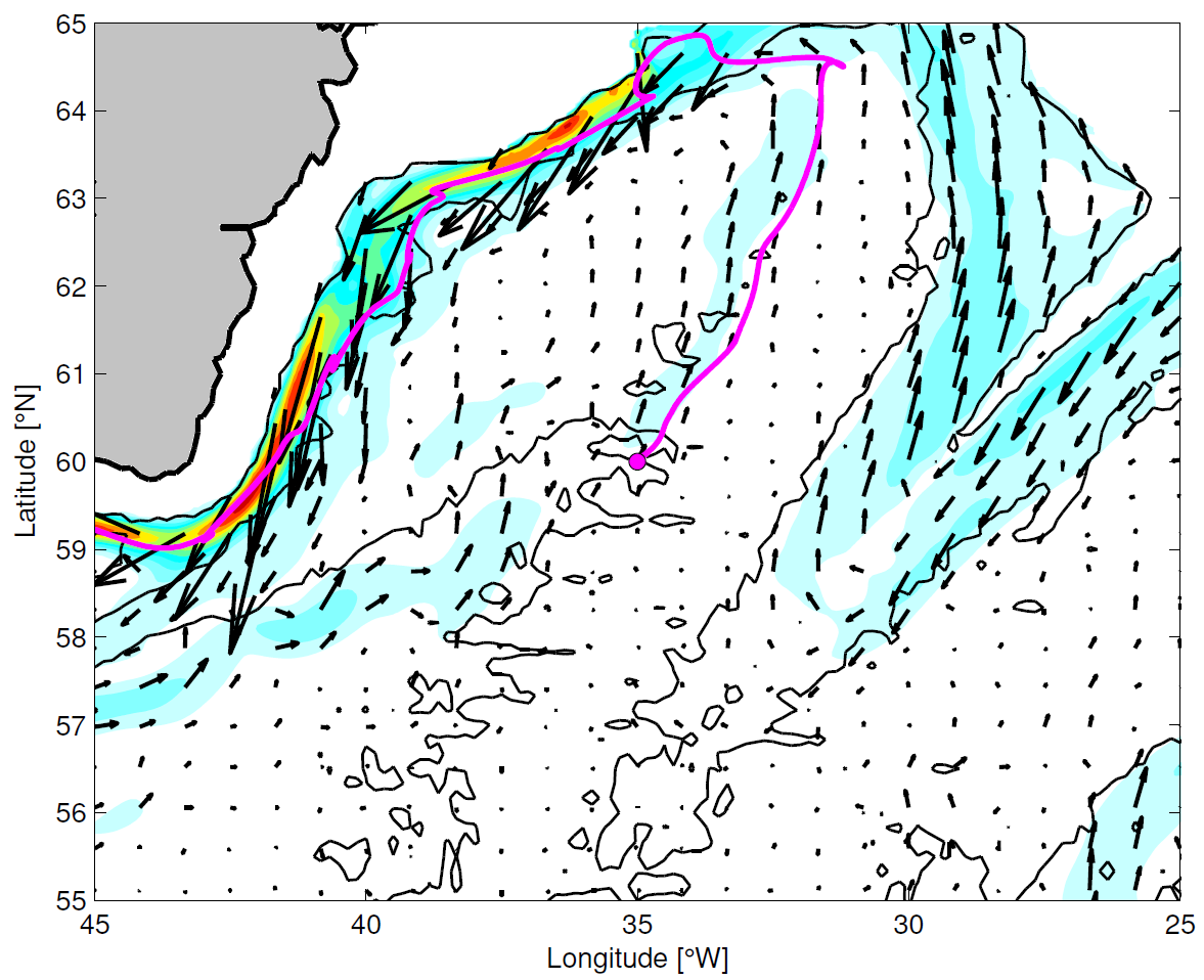
The model’s mean flow. The colors indicate flow speed, from white (zero) to red (“fast” 50 cm/s). The arrows indicate direction as well as speed. The magenta line is the track of a “virtual RAFOS” launched in the mean flow. It starts at the magenta dot.
If you “deploy” a RAFOS on a fixed point in this flow field is will take the same path no matter at which time you deploy it because the flow field doesn’t change. This is what oceanographers in the early days expected to happen in the real ocean as well. Of course, they didn’t have the measurements we have now. The first current meters only counted the number of rotations the propeller made during the deployment. The oceanographer would get the speed by dividing the number of rotations by the time the instrument had been deployed. This gave them the mean speed, but no information about the variability of the flow field. They got the direction of the currents by sending down a compass filled with a liquid that would gradually set and fix the compass’ needle in place.
We know now that the ocean is highly variable and that the mean speed doesn’t give you the total picture. Consider the plot below. It shows the tracks of 12 virtual RAFOS floats deployed in the model field. This time we use the model field that changes every three days and we launch the floats each January 1st. The tracks in this figure show a very different picture than the magenta line before.
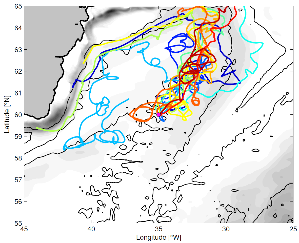
Tracks of 12 virtual RAFOS deployed at the same location as in the previous plot. For these deployments we used the time varying model flow field. Each RAFOS is launched on January 1st of consecutive years. The grey shading indicates where the model flow field is most variable.
Tracks of 12 virtual RAFOS deployed at the same location as in the previous plot. For these deployments we used the time varying model flow field. Each RAFOS is launched on January 1st of consecutive years. The grey shading indicates where the model flow field is most variable.
The RAFOS floats are swirled around by the eddies and each float takes a completely different path, even though they are launched at the same spot (just not at the same time). The much larger area covered by the floats on the eastern side of the basin is an indication that a lot of mixing between water masses may take place there. Also, these RAFOS (which covered one year in both plots) don’t quite get as far as the RAFOS released in the mean flow. It ended up at 60.6 ?N and 58.4 ?W, well outside of the plot. This matter because a parcel of water that starts out warm and travels through colder water will lose a lot more heat if it has to take a longer path to get somewhere.
In two years’ time the real RAFOS we deployed during this cruise will show us the actual underwater pathways. RAFOS deployed in 2014 and those that will be deployed in 2016 will show us how those pathways vary from year to year. Maybe it will look like the model. Maybe not…