By Chris Wilson and Neill Mackay
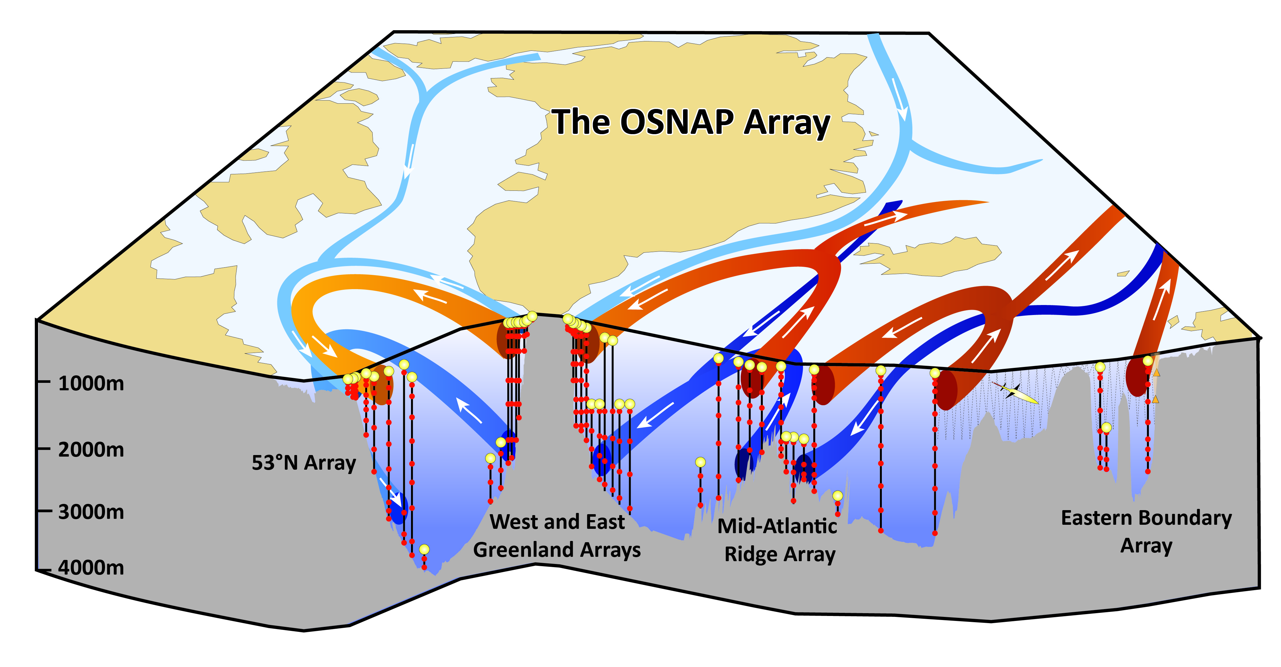
Figure 1: A schematic of the OSNAP array. (Credit: Penny Holliday).
The OSNAP array (Figure 1) will sample what is effectively a two-dimensional ‘slice’ of the ocean for several years at high spatial and temporal frequency. Of course, as shown in Figure 1, the ocean circulation is three-dimensional, and it varies in time. It contains a range of dynamical scales, from millimeters to millennia. As well as understanding the observations in the OSNAP array ‘slice’, our aim is to build a more complete picture of the circulation and to be able to make statistically robust statements about its variability in a changing climate. For example, is a change measured by the array over, say, a few months representative of a larger branch of the North Atlantic circulation, is it a response to external forcing or is it simply due to local intrinsic nonlinear variability?
This observational paradigm is analogous to our exploration of Mars with robotic rovers. Scientists have developed theories describing the wider region based on their best understanding from previous, often sparse, observations. Then a much improved set of observations becomes available, gradually imaging a localised region of the system in fine detail and whose analysis either supports or refutes the existing theories. Only by combining the new, local observations with other, broader observations and estimates, may the best view of the full, three-dimensional system be developed.
Such estimates fall into two categories: solutions to ‘forward’ or ‘inverse’ problems. In each case, there are mathematical equations describing the physics that govern the system (related to fluid mechanics and thermodynamics).
For the ‘forward’ problem, the input is typically some estimate of the initial state of the system and the goal is to find, over a region of time and space, a three-dimensional solution that matches the two-dimensional slice observed by the OSNAP array. A typical example of a ‘forward’ model is a numerical ocean model that is integrated forwards in time. However, it is notoriously difficult to guess the optimal initial conditions that produce a simulation that closely matches the observations. The nonlinear nature of the fluid dynamics means that small uncertainties in initial conditions, boundary forcing (e.g. surface heat or freshwater fluxes) or uncertainties in the governing equations themselves, may lead to a drift away from observations.
For the steady state ‘inverse’ problem, the input is the observations (complete with error estimates) and the desired solutions contain properties of the system buy cialis online that are physically interesting (e.g. large scale ocean currents and their heat transport). The inverse solutions may provide additional spatial structure to the observations, through assumption of geostrophic or hydrostatic balance, or conservation of properties like potential vorticity. Various approaches, such as the Box (Wunsch, 1978), Beta spiral (Schott and Stommel, 1978), Bernoulli (Killworth, 1986) or Tracer-Contour (Zika et al., 2010) ‘inverse methods’ have been developed to solve ocean inverse problems, especially inverse problems which do not have unique solutions. Like numerical ocean models, these inverse methods have different assumptions or governing equations embedded in them. Usually, the aim of inverse methods is to minimise the misfit between the solution and observations, i.e. to generate the most consistent solution.
With our colleague, Jan Zika, we have begun to apply the Tracer-Contour Inverse Method (Figure 2) – to the North Atlantic in order to understand the OSNAP array observations. Initially, we are using complementary observations from Argo floats (http://www.argo.ucsd.edu) to estimate the circulation. The Argo dataset covers a broader spatio-temporal region than the OSNAP array but does not have its uniformly fine sampling resolution.
The goal within OSNAP is to use a wide range of complementary techniques, including both forward methods and inverse methods, to understand and contextualise the observations from the OSNAP array. Through this diverse approach, we will produce the most statistically robust solutions for the ocean circulation.
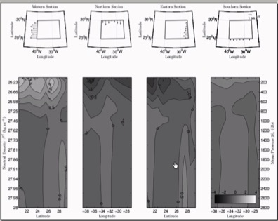
Figure 2. An example of the Tracer-Contour Inverse Method (TCIM) solution for a test volume in the North Atlantic. Lower panels show the velocity component normal to each of the four boundary sections of the test volume (cm/s). The vertical coordinate is neutral density and its equivalent layer-mean pressure is shown on the right axis. Upper panels show the depth-mean of these currents. TCIM also diagnoses estimates of isopycnal and vertical mixing that could help us to find mixing hotspots and to improve models of climate. (Credit: Jan Zika).
Killworth, P. D. (1986), A Bernoulli inverse method for determining the ocean circulation, J. Phys. Oceanogr., 16(12), 2031–2051.
Schott, F., and H. Stommel (1978), Beta spirals and absolute velocities in different oceans, Deep Sea Res. Part I, 25(11), 961–1010, doi:10.1016/0146-6291(78)90583-0.
Wunsch, C. (1978), The North Atlantic general circulation west of 50 W determined by inverse methods, Rev. Geophys., 16(4), 583–620.
Zika, J. D., T. J. Mcdougall, and B. M. Sloyan (2010), A Tracer-Contour Inverse Method for Estimating Ocean Circulation and Mixing, J. Phys. Oceanogr., 40(1), 26–47, doi:10.1175/2009JPO4208.1.